
Fitting a line to data - a quick tutorial
Boris Leistedt, August 2017
This notebook is available at this location on Github.
It is the material presented at a tutorial session at AstroHackWeek 2017. It assumes some basic knowledge about Bayesian inference and data analysis. It is not meant to be standalone since there isn’t much text and it was accompanied by a theory lecture led by Jake Vanderplas. Some good resources on this topic are here, here and here.
%matplotlib inline
%config IPython.matplotlib.backend = 'retina'
%config InlineBackend.figure_format = 'retina'

from IPython.display import HTML
This is a tutorial session.
Don’t be like

Play with the code! Try and do the exercises.
Please interrupt me if you are lost or if you disagree with what I say.
All questions are welcome, especially the ones that you find “simple”, because 1) they are probably not simple, 2) other people are probably wondering the same, 3) they often are the most relevant contributions
If you haven’t done it, install those packages using conda and/or pip:
conda install numpy scipy pandas matplotlib jupyter pip
pip install emcee corner
start a jupyter kernel: jupyter notebook
and open a copy of this notebook.
import matplotlib
import matplotlib.pyplot as plt
from cycler import cycler
matplotlib.rc("font", family="serif", size=14)
matplotlib.rc("figure", figsize="10, 5")
colors = ['k', 'c', 'm', 'y']
matplotlib.rc('axes', prop_cycle=cycler("color", colors))

import scipy.optimize
import numpy as np
Why Bayesian inference?

Road map and Poll
This notebook covers the following topics:
-
Fitting a line to data with y errors.
-
Basics of Bayesian inference and MCMC: gridding, rejection sampling, Metropolis Hastings, convergence, etc.
-
Fitting a line to data with x and y errors. Marginalization of latent variables.
-
Hamiltonian montecarlo for high-dimensional inference. Fitting multiple lines to data (multi-component models). Nested sampling for multimodal solutions. Not covered here: see ixkael.com
Let’s put more weight on some of them according to your demands.
Fitting a line to data
See Hogg, Bovy and Lang (2010): https://arxiv.org/abs/1008.4686
Let’s generate a model:
ncomponents = 1
slopes_true = np.random.uniform(0, 1, ncomponents)
intercepts_true = np.random.uniform(0, 1, ncomponents)
component_fractionalprobs = np.random.dirichlet(np.arange(1., ncomponents+1.))
print('Slopes:', slopes_true)
print('Intercepts:', intercepts_true)
print('Fractional probabilities:', component_fractionalprobs)
# This notebook is ready for you to play with 2+ components and more complicated models.
Slopes: [ 0.55875633]
Intercepts: [ 0.89918981]
Fractional probabilities: [ 1.]
Let’s generate some data drawn from that model:
ndatapoints = 20
xis_true = np.random.uniform(0, 1, ndatapoints)
x_grid = np.linspace(0, 1, 100)

numberpercomponent = np.random.multinomial(ndatapoints, component_fractionalprobs)
print('Number of objects per component:', numberpercomponent)
allocations = np.concatenate([np.repeat(i, nb).astype(int)
                              for i, nb in enumerate(numberpercomponent)])
np.random.shuffle(allocations)
print('Component allocations:', allocations)

def model_linear(xs, slope, intercept): return xs * slope + intercept
yis_true = model_linear(xis_true, slopes_true[allocations], intercepts_true[allocations])
Number of objects per component: [20]
Component allocations: [0 0 0 0 0 0 0 0 0 0 0 0 0 0 0 0 0 0 0 0]
sigma_yis = np.repeat(0.1, ndatapoints) * np.random.uniform(0.5, 2.0, ndatapoints)
yis_noisy = yis_true + np.random.randn(ndatapoints) * sigma_yis
y_min, y_max = np.min(yis_noisy - sigma_yis), np.max(yis_noisy + sigma_yis)
for i in range(ncomponents):
    y_min = np.min([y_min, np.min(model_linear(x_grid, slopes_true[i], intercepts_true[i]))])
    y_max = np.max([y_max, np.max(model_linear(x_grid, slopes_true[i], intercepts_true[i]))])
for i in range(ncomponents):
    plt.plot(x_grid, model_linear(x_grid, slopes_true[i], intercepts_true[i]), c=colors[i])
    ind = allocations == i
    plt.errorbar(xis_true[ind], yis_noisy[ind], sigma_yis[ind], fmt='o', c=colors[i])
plt.xlabel('$$x$$'); plt.ylabel('$$y$$'); plt.ylim([y_min, y_max])
(0.67842208667320758, 1.6708167146558366)
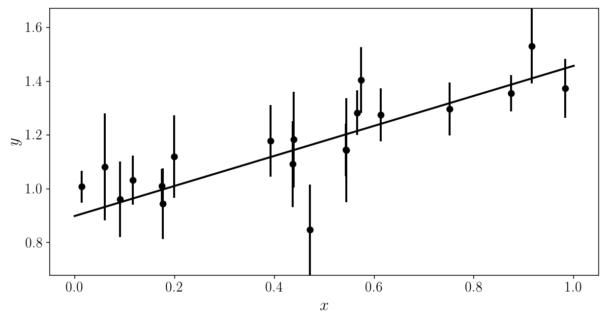
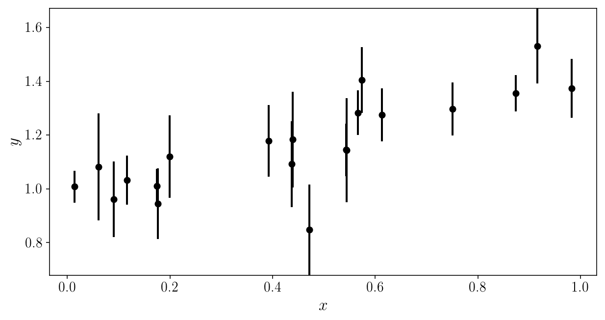
We are going to pretend we don’t know the true model.
Forget what you saw (please).
Here is the noisy data to be analyzed. Can you (mentally) fit a line through it?
plt.errorbar(xis_true, yis_noisy, sigma_yis, fmt='o')
plt.xlabel('$$x$$'); plt.ylabel('$$y$$'); plt.ylim([y_min, y_max])
(0.67842208667320758, 1.6708167146558366)
Let’s define a loss/cost function: the total weighted squared error, also called chi-squared: \(\chi^2 = \sum_i \left( \frac{ \hat{y}_i - y_i^\mathrm{mod}(x_i, s, m) }{\sigma_i} \right)^2\)
def loss(observed_yis, yi_uncertainties, model_yis):
    scaled_differences = (observed_yis - model_yis) / yi_uncertainties
    return np.sum(scaled_differences**2, axis=0)
We want to minimize this chi-squared to obtain the best possible fit to the data.
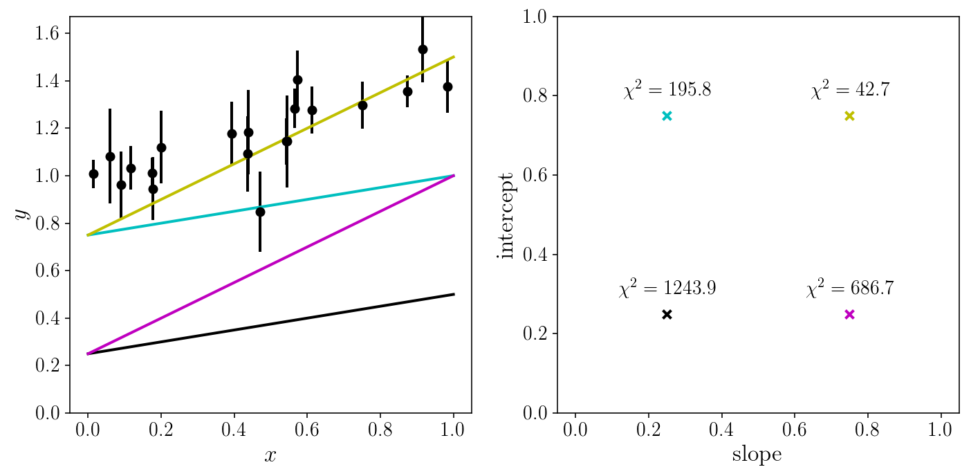
Let us look at the fit for a couple of (random) sets of parameters.
random_slopes = np.array([0.25, 0.25, 0.75, 0.75])
random_intercepts = np.array([0.25, 0.75, 0.25, 0.75])
fig, axs = plt.subplots(1, 2, sharex=True)
axs[0].errorbar(xis_true, yis_noisy, sigma_yis, fmt='o')
for i, (slope, intercept) in enumerate(zip(random_slopes, random_intercepts)):
    axs[0].plot(x_grid, model_linear(x_grid, slope, intercept), c=colors[i])
    axs[1].scatter(slope, intercept,marker='x', c=colors[i])
    chi2 = loss(yis_noisy[:, None], sigma_yis[:, None],
                 model_linear(xis_true[:, None], slope, intercept))
    axs[1].text(slope, intercept+0.05, '$$\chi^2 = %.1f$$'% chi2,
                horizontalalignment='center')
axs[0].set_xlabel('$$x$$'); axs[0].set_ylabel('$$y$$')
axs[0].set_ylim([0, y_max]); axs[1].set_ylim([0, 1]);
axs[1].set_xlabel('slope'); axs[1].set_ylabel('intercept')
fig.tight_layout()
Let us try a brute-force search, and grid our 2D parameter space.
EXERCISE
Create a 100 x 100 grid covering our parameter space.
Evaluate the loss function on the grid, and plot exp(-0.5*loss).
Also find the point that has the minimal loss value.
# SOLUTION
slope_grid, intercept_grid = np.meshgrid(np.linspace(0, 1, 100),
                                         np.linspace(0, 1, 100))
#np.mgrid[0:1:100j, 0:1:100j]
model_yis = model_linear(xis_true[:, None],
                         slope_grid.ravel()[None, :],
                         intercept_grid.ravel()[None, :])
loss_grid = loss(yis_noisy[:, None], sigma_yis[:, None], model_yis[:, :])
# Let's also find the grid point with minimum chi2:
ml_position = np.argmin(loss_grid)
slope_ml = slope_grid.ravel()[ml_position]
intercept_ml = intercept_grid.ravel()[ml_position]
loss_grid = loss_grid.reshape(slope_grid.shape)
fig, axs = plt.subplots(1, 2, sharex=False, sharey=False)
axs[0].errorbar(xis_true, yis_noisy, sigma_yis, fmt='o')
axs[0].plot(x_grid, model_linear(x_grid, slope_ml, intercept_ml))
axs[0].set_xlabel('$$x$$'); axs[0].set_ylabel('$$y$$')
axs[0].set_ylim([y_min, y_max])
axs[1].set_xlabel('slope'); axs[1].set_ylabel('intercept')
axs[1].axvline(slope_ml, c=colors[1]); axs[1].axhline(intercept_ml, c=colors[1])
axs[1].pcolormesh(slope_grid, intercept_grid, np.exp(-0.5*loss_grid), cmap='ocean_r')
fig.tight_layout()
Why visualize \(exp(-\frac{1}{2}\chi^2)\) and not simply the \(\chi^2\)?
Because the former is proportional to our likelihood:
\[\begin{align} p(D| P, M) &= p(\{ \hat{y}_i \} \vert \{\sigma_i, x_i\}, \textrm{intercept}, \textrm{slope}) \\ &= \prod_{i=1}^{N} p(\hat{y}_i \vert x_i, \sigma_i, b, m)\\ &= \prod_{i=1}^{N} \mathcal{N}\left(\hat{y}_i - y^\mathrm{mod}(x_i; m, b); \sigma^2_i \right) \ = \prod_{i=1}^{N} \mathcal{N}\left(\hat{y}_i - m x_i - b; \sigma^2_i \right) \\ &= \prod_{i=1}^{N} \frac{1}{\sqrt{2\pi}\sigma_i}\exp\left( - \frac{1}{2} \frac{(\hat{y}_i - m x_i - b)^2}{\sigma^2_i} \right) \\ &\propto \ \exp\left( - \sum_{i=1}^{N} \frac{1}{2} \frac{(\hat{y}_i - m x_i - b)^2}{\sigma^2_i} \right) \ = \ \exp\left(-\frac{1}{2}\chi^2\right) \end{align}\]Since the data points are independent and the noise is Gaussian.
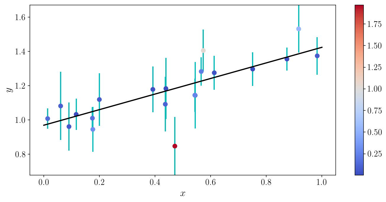
Let’s visualize the \(\chi^2\) for individual objects
model_yis = model_linear(xis_true, slope_ml, intercept_ml)
object_chi2s = 0.5*((yis_noisy - model_yis) / sigma_yis)**2
fig, ax = plt.subplots(1, 1)
ax.plot(x_grid, model_linear(x_grid, slope_ml, intercept_ml))
v = ax.scatter(xis_true, yis_noisy, c=object_chi2s, cmap='coolwarm', zorder=0)
ax.errorbar(xis_true, yis_noisy, sigma_yis, fmt='o', zorder=-1)
ax.set_xlabel('$$x$$'); ax.set_ylabel('$$y$$'); ax.set_ylim([y_min, y_max])
plt.colorbar(v); fig.tight_layout()
Digression
Is a line a good model?
Should we aiming at maximizing the likelihood only?
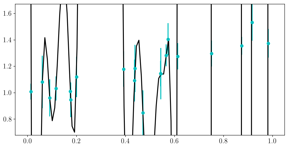
Here is a danger of Maximum Likelihood: there is always of model that perfectly fits all of the data.
This model does not have to be complicated…
EXERCISE (5 min): can you try to write a very flexible model that fits the data perfectly, i.e. go through every single point? What \(\chi^2\) does it lead to?
NOTE: this might not be trivial, so just look for a model that goes through most of the data points.
HINT: numpy has good infrastructure for constructing and fitting polynomials… (try ?np.polyfit).
If you pick a more complicated model you might need to use scipy.optimize.minimize.
# SOLUTION
degree = 150
bestfit_polynomial_coefs = np.polyfit(xis_true, yis_noisy, degree)
bestfit_polynomial = np.poly1d(bestfit_polynomial_coefs)
chi2 = loss(yis_noisy, sigma_yis, bestfit_polynomial(xis_true))
print('The chi2 is', chi2)
The chi2 is 2.08148768845e-05


/Users/bl/anaconda/lib/python3.5/site-packages/ipykernel/__main__.py:3: RankWarning: Polyfit may be poorly conditioned
  app.launch_new_instance()
plt.plot(x_grid, bestfit_polynomial(x_grid))
plt.errorbar(xis_true, yis_noisy, sigma_yis, fmt='o')
plt.ylim([y_min, y_max])
(0.67842208667320758, 1.6708167146558366)
 Copyright Daniela Huppenkothen, Astrohackweek 2015 in NYC
Bayes’ theorem
with explicit Model and Fixed parameters conditioned on:
\[p(P | D, M, F) = \frac{p(D | P, M, F)\ p(P | M, F)}{p(D | M, F)}\]In our case, if we omit the explicit dependence on a linear model:
\[p\bigl(m, s \ \bigl\vert \ \{ \hat{y}_i, \sigma_i, x_i\} \bigr) \ \propto \ p\bigl(\{ \hat{y}_i \} \ \bigl\vert \ m, s, \{\sigma_i, x_i\}\bigr) \ p\bigl(m, s\bigr) \ = \ \exp\bigl(-\frac{1}{2}\chi^2\bigr)\ p\bigl(m, s\bigr)\]# Let us play with Bayes theorem and pick some un-motivated prior:
prior_grid = np.exp(-slope_grid**-1) * np.exp(-intercept_grid**-1)
likelihood_grid = np.exp(-0.5*loss_grid)
posterior_grid = likelihood_grid * prior_grid
/Users/bl/anaconda/lib/python3.5/site-packages/ipykernel/__main__.py:2: RuntimeWarning: divide by zero encountered in reciprocal
  from ipykernel import kernelapp as app
fig, axs = plt.subplots(1, 3)
for i in range(3):
    axs[i].set_ylabel('intercept'); axs[i].set_xlabel('slope');
axs[0].set_title('Prior'); axs[1].set_title('Likelihood'); axs[2].set_title('Posterior')
axs[1].axvline(slope_ml, c=colors[1]); axs[1].axhline(intercept_ml, c=colors[1])
axs[0].pcolormesh(slope_grid, intercept_grid, prior_grid, cmap='ocean_r')
axs[1].pcolormesh(slope_grid, intercept_grid, likelihood_grid, cmap='ocean_r')
axs[2].pcolormesh(slope_grid, intercept_grid, posterior_grid, cmap='ocean_r')
fig.tight_layout()
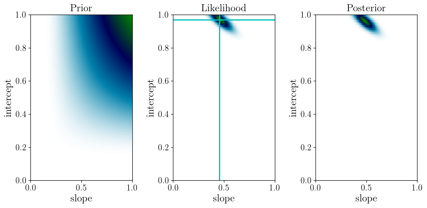
Discussion: what priors are adequate here?
Three common types of priors are:
- Empirical priors
- Conjugate priors
- Flat priors
- Non-informative priors
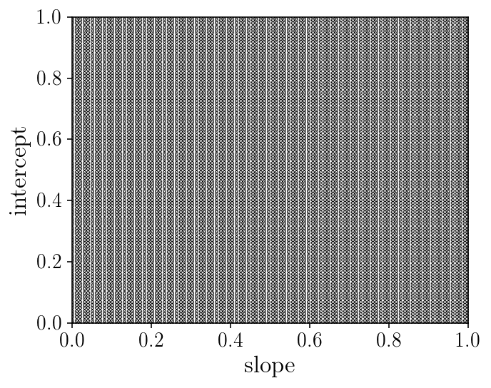
The Curse of Dimensionality (v1)
Problems with ‘gridding’: number of likelihood evaluations, resolution of the grids, etc
fig, ax = plt.subplots(1, 1, figsize=(5, 4))
ax.set_xlabel('slope'); ax.set_ylabel('intercept');
ax.scatter(slope_grid.ravel(), intercept_grid.ravel(), marker='.', s=1)
ax.set_ylim([0, 1])
ax.set_xlim([0, 1])
fig.tight_layout()
print('Number of point/evaluations of the likelihood:', slope_grid.size)
Number of point/evaluations of the likelihood: 10000
Sampling posterior distributions with MCMC
We are going to approximate the posterior distribution with a set of samples.
EXERCISE
Write three functions returning:
-
the log of the likelihood
ln_like(params, args...). -
the log of the prior
ln_prior(params, args...). -
the log of the posterior
ln_post(params, args...).
The likelihood is pretty much our previous loss function.
The prior should return -np.inf outside of our parameter space of interest. At this stage use a uniform prior in \([0, 1] \times [0, 1]\).
Think about what other priors could be used. Include the correct normalization in the prior and the likelihood if possible.
def ln_like(params, xs, observed_yis, yi_uncertainties):
    model_yis = model_linear(xs, params[0], params[1])
    chi2s = ((observed_yis - model_yis) / yi_uncertainties)**2
    return np.sum(-0.5 * chi2s - 0.5*np.log(2*np.pi) - np.log(yi_uncertainties))

def ln_prior(params):
    if np.any(params < 0) or np.any(params > 1):
        return - np.inf
    return 0.

def ln_post(params, xs, observed_yis, yi_uncertainties):
    lnprior_val = ln_prior(params)
    if ~np.isfinite(lnprior_val):
        return lnprior_val
    else:
        lnlike_val = ln_like(params, xs, observed_yis, yi_uncertainties)
        return lnprior_val + lnlike_val
x0 = np.array([0.5, 0.5])
print('Likelihood:', ln_like(x0, xis_true, yis_noisy, sigma_yis))
print('Prior:', ln_prior(x0))
print('Posterior:', ln_post(x0, xis_true, yis_noisy, sigma_yis))
Likelihood: -170.940432172
Prior: 0.0
Posterior: -170.940432172
EXERCISE (2 min)
Find the maximum of the log posterior. Try different optimizers in scipy.optimize.minimize. Be careful about the sign of the objective function (is it plus or minus the log posterior?)
# SOLUTION
def fun(p0):
    return - ln_post(p0, xis_true, yis_noisy, sigma_yis)

res = scipy.optimize.minimize(fun, np.random.uniform(0, 1, 2), method='Powell')
print(res)
best_parmas = res.x
   direc: array([[-0.00510155,  0.0181219 ],
       [-0.25753496,  0.1202727 ]])
     fun: -19.208039955530083
 message: 'Optimization terminated successfully.'
    nfev: 102
     nit: 4
  status: 0
 success: True
       x: array([ 0.45976482,  0.96643451])


/Users/bl/anaconda/lib/python3.5/site-packages/scipy/optimize/optimize.py:1850: RuntimeWarning: invalid value encountered in double_scalars
  tmp2 = (x - v) * (fx - fw)
/Users/bl/anaconda/lib/python3.5/site-packages/scipy/optimize/optimize.py:2189: RuntimeWarning: invalid value encountered in double_scalars
  w = xb - ((xb - xc) * tmp2 - (xb - xa) * tmp1) / denom
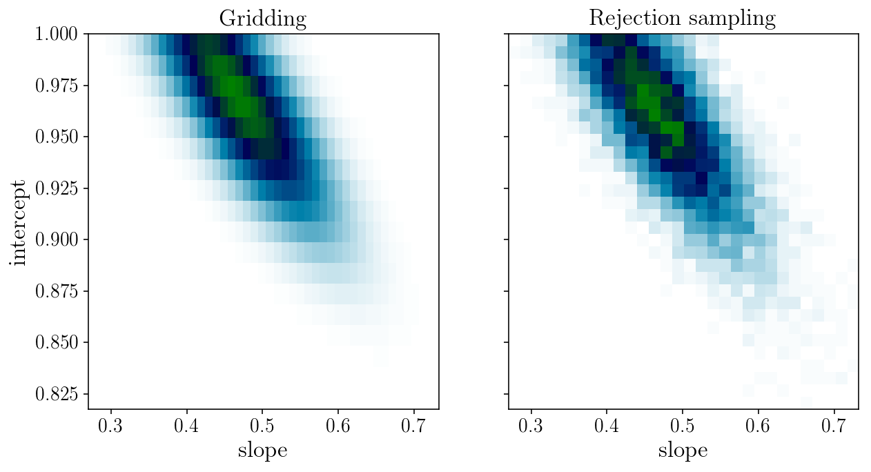
Sampling strategy 1: Rejection Sampling
EXERCISE
Implement rejection sampling. Randomly draw points in our 2D parameter space. Keep each point with a probability proportional to the posterior distribution.
HINT: you will find that you need to normalize the posterior distribution in some way to make the sampling possible. Use the MAP solution we just found!
# SOLUTION
normalization = ln_post(best_parmas, xis_true, yis_noisy, sigma_yis)
print(normalization)
num_draws = 10000
i_draw = 0
params_drawn = np.zeros((num_draws, 2))
params_vals = np.zeros((num_draws, ))
num_tot = 0
while i_draw < num_draws:
    params_drawn[i_draw, :] = np.random.uniform(0, 1, 2)
    params_vals[i_draw] = np.exp(
        ln_post(params_drawn[i_draw, :], xis_true, yis_noisy, sigma_yis)\
        - normalization)
    num_tot += 1
    if np.random.uniform(0, 1, 1) < params_vals[i_draw]:
        #print(params_vals[i_draw], i_draw)
        i_draw += 1
print(num_tot, num_draws)
19.2080399555
1184302 10000
fig, axs = plt.subplots(1, 2, sharex=True, sharey=True)
axs[0].pcolormesh(slope_grid, intercept_grid, likelihood_grid, cmap='ocean_r')
axs[1].hist2d(params_drawn[:, 0], params_drawn[:, 1], 30, cmap="ocean_r");
axs[0].set_title('Gridding'); axs[1].set_title('Rejection sampling');
axs[0].set_xlabel('slope'); axs[0].set_ylabel('intercept'); axs[1].set_xlabel('slope');
Sampling strategy 2: Metropolis-Hastings
The Metropolis-Hastings algorithm
For a given target probability \(p(\theta)\) and a (symmetric) proposal density \(p(\theta_{i+1}|\theta_i)\). We repeat the following:
- draw a sample \(\theta_{i+1}\) given \(\theta_i\) from the proposal density,
- compute the acceptance probability ratio \(a={p(\theta_{i+1})}/{p(\theta_i)}\),
- draw a random uniform number \(r\) in \([0, 1]\) and accept \(\theta_{i+1}\) if \(r < a\).
EXERCISE
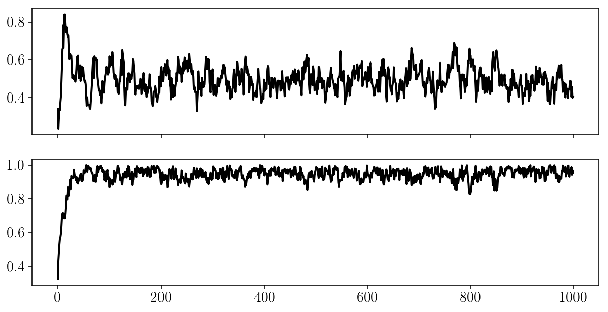
Use your implementation of the Metropolis-Hastings algorithm to draw samples from our 2D posterior distribution of interest.
Measure the proportion of parameter draws that are accepted: the acceptance rate.
Plot the chain and visualize the burn-in phase.
Compare the sampling to our previous gridded version.
Estimate the mean and standard deviation of the distribution from the samples. Are they accurate?
# SOLUTION
num_draws = 1000
params_drawn = np.zeros((num_draws, 2))
i_draw = 1
num_draws_tot = 0
params_drawn[0, :] = np.random.uniform(0, 1, 2)
while i_draw < num_draws:
    num_draws_tot += 1
    params_drawn[i_draw, :] = params_drawn[i_draw-1, :] \
        + 0.05 * np.random.randn(2)
    a = np.exp(ln_post(params_drawn[i_draw, :], xis_true, yis_noisy, sigma_yis)\
                   - ln_post(params_drawn[i_draw-1, :], xis_true, yis_noisy, sigma_yis))
    if a >= 1 or np.random.uniform(0, 1, 1) < a:
        i_draw += 1
print('Acceptance rate:', num_draws/num_draws_tot)
Acceptance rate: 0.3721622627465575
fig, axs = plt.subplots(1, 2, sharex=True, sharey=True)
axs[0].pcolormesh(slope_grid, intercept_grid, likelihood_grid, cmap='ocean_r')
axs[1].hist2d(params_drawn[:, 0], params_drawn[:, 1], 30, cmap="ocean_r");
axs[0].set_xlabel('slope'); axs[0].set_ylabel('intercept'); axs[1].set_xlabel('slope');
fig, ax = plt.subplots(2, sharex=True)
for i in range(2):
    ax[i].plot(params_drawn[:, i]);
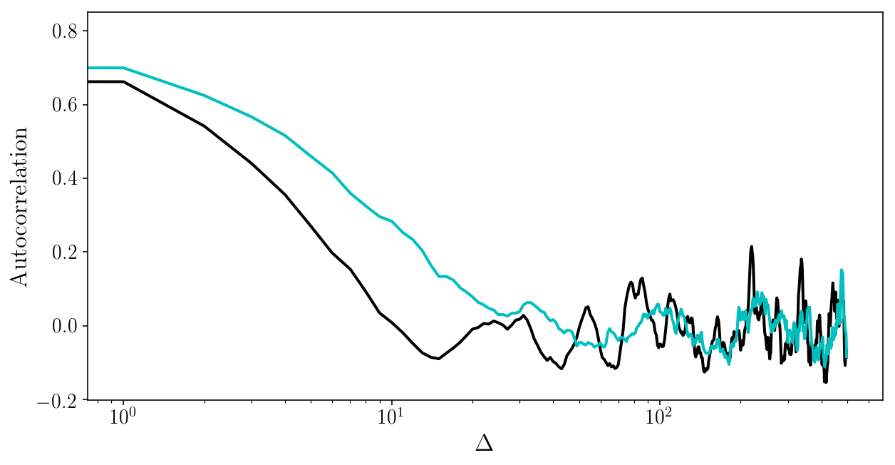
Validation
MCMC is approximate and is only valid if it has converged. But we can’t prove that a chain has converget - we can only show it hasn’t.
What to do? _Be paranoïd.
Is it crucial to 1) run many chains in various setups, and 2) check that the results are stable, and 3) look at the auto-correlation time:
\[\rho_k = \frac{\mathrm{Covar}[X_t, X_{t+k}]}{\mathrm{Var}[X_t]\mathrm{Var}[X_{t+k}]]}\]See http://rstudio-pubs-static.s3.amazonaws.com/258436_5c7f6f9a84bd47aeaa33ee763e57a531.html and www.astrostatistics.psu.edu/RLectures/diagnosticsMCMC.pdf
EXERCISE
Visualize chains, autocorrelation time, etc, for short and long chains with different proposal distributions in the Metropolis Hastings algorithm.
# SOLUTION
def autocorr_naive(chain, cutoff):
    auto_corr = np.zeros(cutoff-1)
    mu = np.mean(chain, axis=0)
    var = np.var(chain, axis=0)
    for s in range(1, cutoff-1):
        auto_corr[s] = np.mean( (chain[:-s] - mu) * (chain[s:] - mu) ) / var
    return auto_corr[1:]
for i in range(2):
plt.plot(autocorr_naive(params_drawn[:, i], 500))
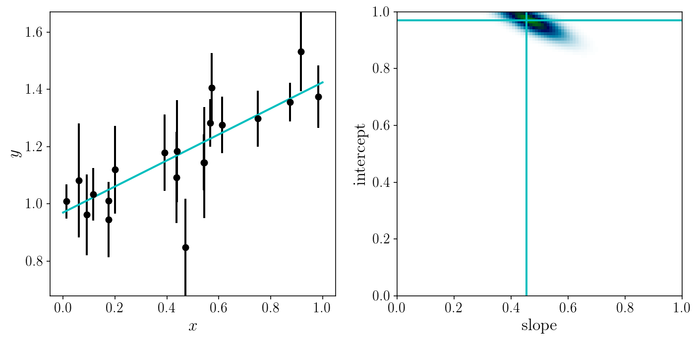
plt.xscale('log'); plt.xlabel('$$\Delta$$'); plt.ylabel('Autocorrelation');
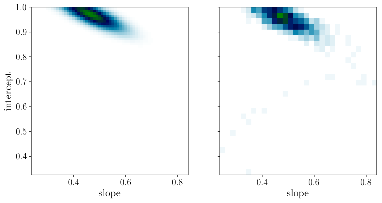
Sampling strategy 3: affine-invariant ensemble sampler
EXERCISE
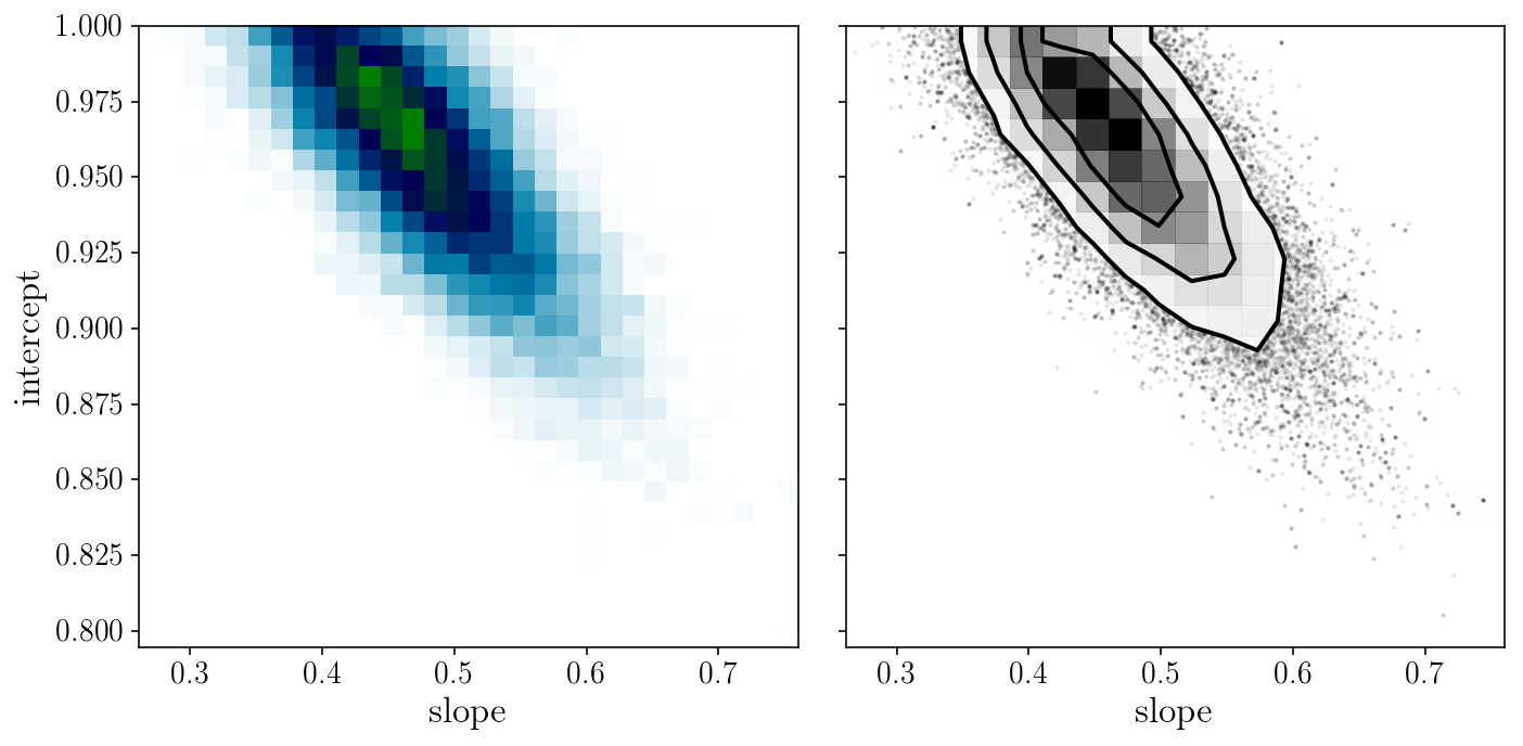
Let’s use a more advanced sampler. Look at the documentation of the emcee package and use it to (again) draw samples from our 2D posterior distribution of interest. Make 2D plots with both plt.hist2d or plt.contourf. For the latter, add 68% and 95% confidence contours.
# SOLUTION
import emcee

ndim = 2
nwalkers = 50

starting_params = np.random.uniform(0, 1, ndim*nwalkers).reshape((nwalkers, ndim))
sampler = emcee.EnsembleSampler(nwalkers, ndim, ln_post,
                                args=[xis_true, yis_noisy, sigma_yis])

num_steps = 100
pos, prob, state = sampler.run_mcmc(starting_params, num_steps)
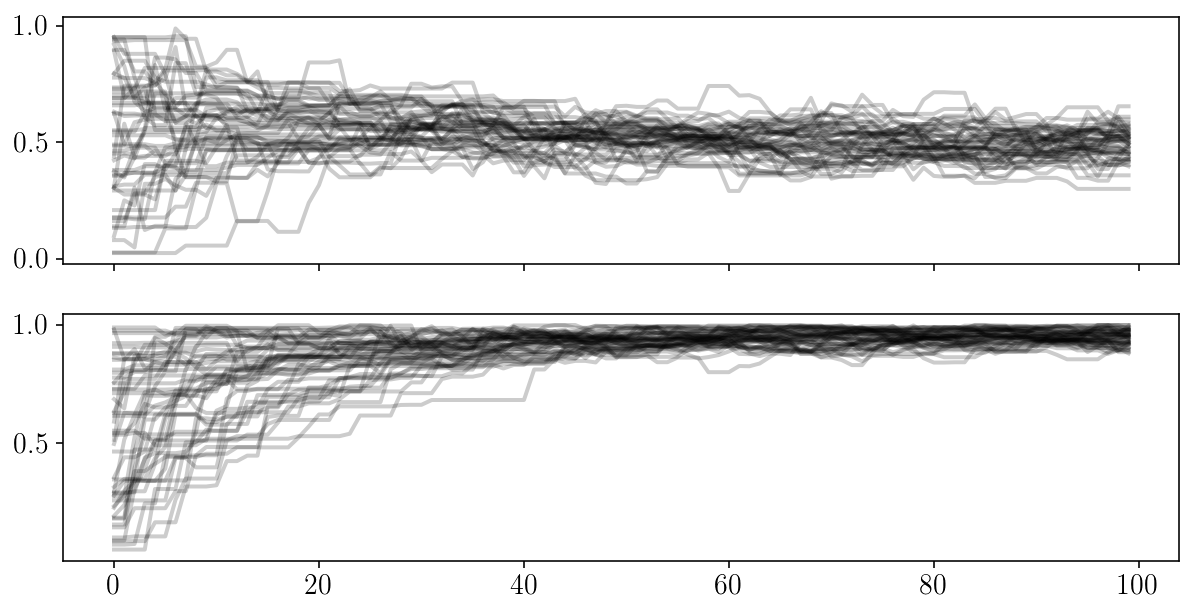
fig, ax = plt.subplots(2, sharex=True)
for i in range(2):
    ax[i].plot(sampler.chain[:, :, i].T, '-k', alpha=0.2);
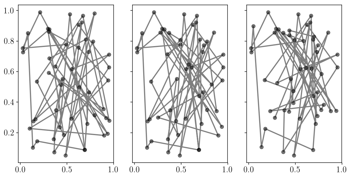
fig, axs = plt.subplots(1, 3, sharex=True, sharey=True)
for i in range(axs.size):
    axs[i].errorbar(sampler.chain[:, i, 0], sampler.chain[:, i, 1], fmt="-o", alpha=0.5, c='k');
num_steps = 1000
sampler.reset()
pos, prob, state = sampler.run_mcmc(pos, num_steps)
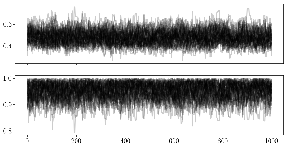
fig, ax = plt.subplots(2, sharex=True)
for i in range(2):
    ax[i].plot(sampler.chain[:, :, i].T, '-k', alpha=0.2);
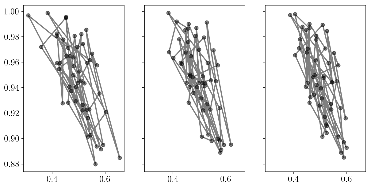
fig, axs = plt.subplots(1, 3, sharex=True, sharey=True)
for i in range(axs.size):
    axs[i].errorbar(sampler.chain[:, i, 0], sampler.chain[:, i, 1], fmt="-o", alpha=0.5, c='k');
from corner import hist2d
fig, axs = plt.subplots(1, 2, sharex=True, sharey=True)
axs[0].hist2d(sampler.flatchain[:, 0], sampler.flatchain[:, 1], 30, cmap="ocean_r");
hist2d(sampler.flatchain[:, 0], sampler.flatchain[:, 1], ax=axs[1])
axs[0].set_xlabel('slope'); axs[0].set_ylabel('intercept'); axs[1].set_xlabel('slope');
fig.tight_layout()
fig, axs = plt.subplots(1, 2, sharex=True, sharey=True)
axs[0].hist(sampler.flatchain[:, 0], histtype='step');
axs[1].hist(sampler.flatchain[:, 1], histtype='step');
axs[0].set_xlabel('slope'); axs[1].set_xlabel('intercept'); axs[0].set_ylabel('Marginal distribution');
fig.tight_layout()

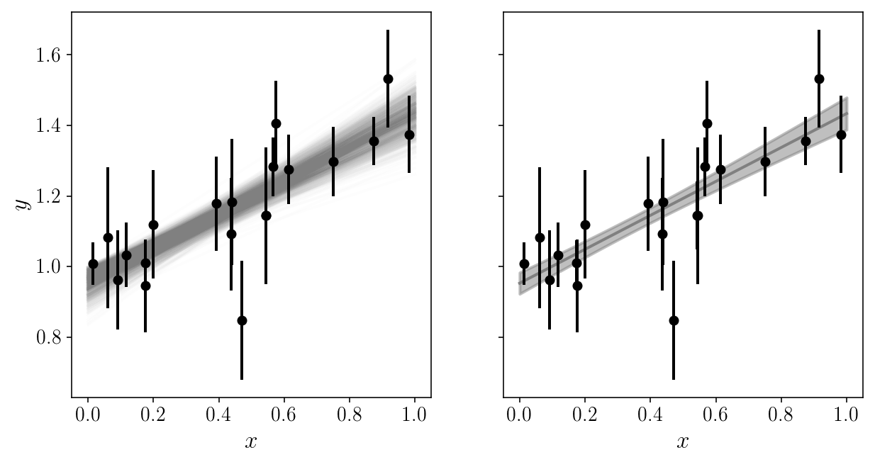
It is extremely useful to plot the model in data space!
EXERCISE
Loop through the posterior samples (a random subset of them?) and over-plot them with the data, with some transparency.
# SOLUTION
fig, axs = plt.subplots(1, 2, sharex=True, sharey=True)
axs[0].set_xlabel('$$x$$'); axs[1].set_xlabel('$$x$$'); axs[0].set_ylabel('$$y$$');
num = 1000
y_models = np.zeros((x_grid.size, num))
for j, i in enumerate(np.random.choice(np.arange(sampler.flatchain.shape[0]), num, replace=False)):
    y_models[:, j] = model_linear(x_grid, sampler.flatchain[i, 0], sampler.flatchain[i, 1])
    axs[0].plot(x_grid, y_models[:, j], c='gray', alpha=0.01, zorder=0)
axs[1].plot(x_grid, np.mean(y_models, axis=1), c='gray', alpha=1, zorder=0)
axs[1].fill_between(x_grid, np.mean(y_models, axis=1)-np.std(y_models, axis=1),
            np.mean(y_models, axis=1)+np.std(y_models, axis=1), color='gray', alpha=0.5, zorder=0)
axs[0].errorbar(xis_true, yis_noisy, sigma_yis, fmt='o', zorder=1)
axs[1].errorbar(xis_true, yis_noisy, sigma_yis, fmt='o', zorder=1)
<Container object of 3 artists>
fig, axs = plt.subplots(1, 2, sharex=True, sharey=True)
axs[0].hist(sampler.flatchain[:, 0], histtype='step');
axs[1].hist(sampler.flatchain[:, 1], histtype='step');
axs[0].set_xlabel('slope'); axs[1].set_xlabel('intercept'); axs[0].set_ylabel('Marginal distribution');
fig.tight_layout()
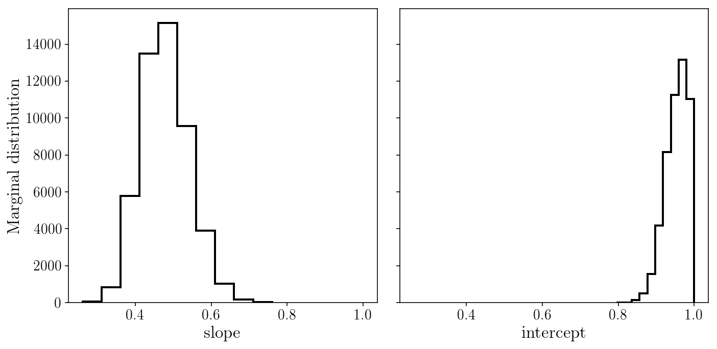
Parameter estimation
Often, we want to report summary statistics on our parameters, e.g. in a paper.
EXERCISE
Compute some useful summary statistics for our two parameters from the MCMC chains: mean, confidence intervals, etc
# SOLUTION
thechain = sampler.flatchain
print('Mean values:', np.mean(thechain, axis=0))
print('Standard deviation:', np.std(thechain, axis=0))
print('Quantiles:', np.percentile(thechain, [5, 16, 50, 84, 95], axis=0))
Mean values: [ 0.47939804  0.95345458]
Standard deviation: [ 0.06201173  0.02980449]
Quantiles: [[ 0.38360387  0.89916009]
 [ 0.41757193  0.92274662]
 [ 0.47588074  0.95753917]
 [ 0.54063416  0.98415853]
 [ 0.58694499  0.99449373]]
NOTE: for any subsequent analysis, don’t use the summary statistics, use the full MCMC chains if you can!
CONTROVERSIAL: if you are only ever going to report and use the mean of a parameter, maybe you don’t need MCMC…
Fitting data with both x and y errors
We observe a set of \(\hat{x}_i\) which are noisified versions of the true \(x_i\), with Gaussian noise \(\gamma_i\).
sigma_xis = np.repeat(0.1, ndatapoints) * np.random.uniform(0.2, 1.0, ndatapoints)
xis_noisy = xis_true + sigma_xis * np.random.randn(xis_true.size)
plt.errorbar(xis_noisy, yis_noisy, xerr=sigma_xis, yerr=sigma_yis, fmt='o')
plt.xlabel('$$x$$'); plt.ylabel('$$y$$'); plt.ylim([y_min, y_max])
(0.67842208667320758, 1.6708167146558366)
Our likelihood is now:
\[\begin{align} p(D| P, M) &= p(\{ \hat{y}_i, \hat{x}_i \} \vert \{\sigma_i, \gamma_i, x_i\}, \textrm{intercept}, \textrm{slope}) \\ &= \prod_{i=1}^{N} p(\hat{y}_i \vert x_i, \sigma_i, b, m) \ p(\hat{x}_i \vert x_i, \gamma_i) \\ & = \prod_{i=1}^{N} \mathcal{N}\left(\hat{y}_i - m x_i - b; \sigma^2_i \right) \mathcal{N}\left(\hat{x}_i - x_i; \gamma^2_i \right) \end{align}\]We now have \(N\) extra parameters, the \(x_i\)’s!
The full posterior distribution:
\[p\bigl( m, s, \{ x_i \} \bigl\vert \{ \hat{y}_i, \hat{x}_i, \sigma_i, \gamma_i\} \bigr) \ \propto \ p\bigl(\{ \hat{y}_i, \hat{x}_i \} \bigl\vert \{\sigma_i, \gamma_i, x_i\}, m, s\bigr) \ \ p\bigl(\{ x_i \}, m, s\bigr)\]This is the Curse of Dimensionality v2!
import autograd.numpy as onp

def ln_like(params, observed_yis, observed_xis, yi_uncertainties, xi_uncertainties):
    model_yis = model_linear(params[2:], params[0], params[1])
    lnlike_yis = onp.sum(-0.5 * ((observed_yis - model_yis) / yi_uncertainties)**2
                   - 0.5*onp.log(2*np.pi) - onp.log(yi_uncertainties))
    lnlike_xis = onp.sum(-0.5 * ((observed_xis - params[2:]) / xi_uncertainties)**2
                   - 0.5*onp.log(2*np.pi) - onp.log(xi_uncertainties))
    return lnlike_yis + lnlike_xis

def ln_prior(params):
    if onp.any(params < 0) or onp.any(params > 1):
        return - onp.inf
    return 0.

def ln_post(params, observed_yis, observed_xis, yi_uncertainties, xi_uncertainties):
    lnprior_val = ln_prior(params)
    if ~onp.isfinite(lnprior_val):
        return lnprior_val
    else:
        lnlike_val = ln_like(params, observed_yis, observed_xis, yi_uncertainties, xi_uncertainties)
        return - lnprior_val - lnlike_val
One solution : Hamiltonian Monte Carlo
Neal’s book chapter is a good starting point: https://arxiv.org/abs/1206.1901
Demo: https://chi-feng.github.io/mcmc-demo/app.html
Gradients (and hessians) needed! Three strategies:
- pen and paper, then home-made implementation
- automatic symbolic differentiation
- automatic numerical differentition
Always try auto-diff first (e.g., with autograd).
Large-scale inference (gazilion parameters): try tensorflow
from autograd import grad, hessian

ln_post_gradient = grad(ln_post)
ln_post_hessian = hessian(ln_post)
x0 = np.repeat(0.5, ndatapoints + 2)
print('Likelihood:', ln_like(x0, yis_noisy, xis_noisy, sigma_yis, sigma_xis))
print('Prior:', ln_prior(x0))
print('Posterior:', ln_post(x0, yis_noisy, xis_noisy, sigma_yis, sigma_xis))
print('Posterior gradient:', ln_post_gradient(x0, yis_noisy, xis_noisy, sigma_yis, sigma_xis))
print('Posterior hessian (diagonal):', np.diag(ln_post_hessian(x0, yis_noisy, xis_noisy, sigma_yis, sigma_xis)))
Likelihood: -479.086846649
Prior: 0.0
Posterior: 479.086846649
Posterior gradient: [-389.59298124 -779.18596249   12.3987198   106.60267919   56.82249183
  -34.18536339  240.3974905   348.68958026 -179.77260948    9.9641432
  -12.90856215  -41.65438946  -59.9212448   -74.3301498   -60.19003428
 -445.3267937   170.61144594   -7.47111959  128.40256476  -67.75092668
  -14.98329646   27.44128385]
Posterior hessian (diagonal): [  470.93448395  1883.73793582   181.81674184   673.15051509   201.64679029
   194.39369459   613.96221224   772.60461028   448.96781047   146.55077539
   121.25587699   254.73967871   324.71339006   135.2362151    171.07058365
  1229.44118614   474.73624695   141.04615414   460.96337899  1879.19300776
   128.96207815   136.9411144 ]
# Simplest implementation of HMC
def hmc_sampler(x0, lnprob, lnprobgrad, step_size, num_steps, args):
    v0 = np.random.randn(x0.size)
    v = v0 - 0.5 * step_size * lnprobgrad(x0, *args)
    x = x0 + step_size * v
    for i in range(num_steps):
        v = v - step_size * lnprobgrad(x, *args)
        x = x + step_size * v
    v = v - 0.5 * step_size * lnprobgrad(x, *args)
    orig = lnprob(x0, *args)
    current = lnprob(x, *args)
    orig += 0.5 * np.dot(v0.T, v0)
    current += 0.5 * np.dot(v.T, v)
    p_accept = min(1.0, np.exp(orig - current))
    if(np.any(~np.isfinite(x))):
        print('Error: some parameters are infinite!')
        print('HMC steps and stepsize:', num_steps, step_size)
        return x0
    if p_accept > np.random.uniform():
        return x
    else:
        if p_accept < 0.01:
            print('Sample rejected due to small acceptance prob (', p_accept, ')')
            print('HMC steps and stepsize:', num_steps, step_size)
        return x0
Analytic marginalization of latent variables
We are only truly interested in the marginalized posterior distribution:
\[p\bigl( m, s \bigl\vert \{ \hat{y}_i, \hat{x}_i, \sigma_i, \gamma_i\} \bigr) \ = \ \int\mathrm{d}\{x_i\} p\bigl( m, s, \{ x_i \} \bigl\vert \{ \hat{y}_i, \hat{x}_i, \sigma_i, \gamma_i\} \bigr) \\ \propto \ \prod_{i=1}^{N} \int \mathrm{d}x_i \mathcal{N}\left(\hat{y}_i - m x_i - b; \sigma^2_i \right) \mathcal{N}\left(\hat{x}_i - x_i; \gamma^2_i \right) \ \ p\bigl(\{ x_i \}, m, s\bigr) \\ \propto \ \prod_{i=1}^{N} \mathcal{N}\left(\hat{y}_i - m \hat{x}_i - b; \sigma^2_i + \gamma^2_i\right) \ p(s, m)\]with flat uninformative priors on \(x_i\)’s \(p\bigl(x_i)\).
We have eliminated the \(x_i\)’s!

def ln_like(params, observed_yis, observed_xis, yi_uncertainties, xi_uncertainties):
    xyi_uncertainties = np.sqrt(xi_uncertainties**2. + yi_uncertainties**2.)
    model_yis = model_linear(observed_xis, params[0], params[1])
    return onp.sum(-0.5 * ((observed_yis - model_yis) / xyi_uncertainties)**2
                   - 0.5*onp.log(2*np.pi) - onp.log(xyi_uncertainties))

def ln_prior(params):
    if np.any(params < 0) or np.any(params > 1):
        return - onp.inf
    return 0.

def ln_post(params, observed_yis, observed_xis, yi_uncertainties, xi_uncertainties):
    lnprior_val = ln_prior(params)
    if ~onp.isfinite(lnprior_val):
        return lnprior_val
    else:
        lnlike_val = ln_like(params, observed_yis, observed_xis, yi_uncertainties, xi_uncertainties)
        return lnprior_val + lnlike_val
x0 = np.repeat(0.5, 2)
print('Likelihood:', ln_like(x0, yis_noisy, xis_noisy, sigma_yis, sigma_xis))
print('Prior:', ln_prior(x0))
print('Posterior:', ln_post(x0, yis_noisy, xis_noisy, sigma_yis, sigma_xis))
Likelihood: -124.693107274
Prior: 0.0
Posterior: -124.693107274
ndim = 2
nwalkers = 50

starting_params = np.random.uniform(0, 1, ndim*nwalkers).reshape((nwalkers, ndim))
sampler2 = emcee.EnsembleSampler(nwalkers, ndim, ln_post,
                                args=[yis_noisy, xis_noisy, sigma_yis, sigma_xis])

num_steps = 100
pos, prob, state = sampler2.run_mcmc(starting_params, num_steps)
num_steps = 1000
sampler2.reset()
pos, prob, state = sampler2.run_mcmc(pos, num_steps)
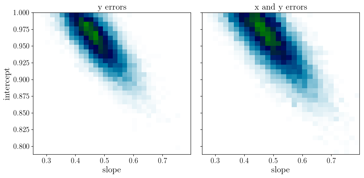
fig, axs = plt.subplots(1, 2, sharex=True, sharey=True)
axs[0].hist2d(sampler.flatchain[:, 0], sampler.flatchain[:, 1], 30, cmap="ocean_r");
axs[1].hist2d(sampler2.flatchain[:, 0], sampler2.flatchain[:, 1], 30, cmap="ocean_r");
axs[0].set_title('y errors'); axs[1].set_title('x and y errors');
axs[0].set_xlabel('slope'); axs[0].set_ylabel('intercept'); axs[1].set_xlabel('slope');
fig.tight_layout()
fig, axs = plt.subplots(1, 2, sharex=True, sharey=True)
axs[0].set_xlabel('$$x$$'); axs[1].set_xlabel('$$x$$'); axs[0].set_ylabel('$$y$$');
num = 1000
y_models = np.zeros((x_grid.size, num))
for j, i in enumerate(np.random.choice(np.arange(sampler2.flatchain.shape[0]), num, replace=False)):
    y_models[:, j] = model_linear(x_grid, sampler2.flatchain[i, 0], sampler2.flatchain[i, 1])
    axs[0].plot(x_grid, y_models[:, j], c='gray', alpha=0.01, zorder=0)
axs[1].plot(x_grid, np.mean(y_models, axis=1), c='gray', alpha=1, zorder=0)
axs[1].fill_between(x_grid, np.mean(y_models, axis=1)-np.std(y_models, axis=1),
            np.mean(y_models, axis=1)+np.std(y_models, axis=1), color='gray', alpha=0.5, zorder=0)
axs[0].errorbar(xis_noisy, yis_noisy, xerr=sigma_xis, yerr=sigma_yis, fmt='o', zorder=1)
axs[1].errorbar(xis_noisy, yis_noisy, xerr=sigma_xis, yerr=sigma_yis, fmt='o', zorder=1)
<Container object of 3 artists>
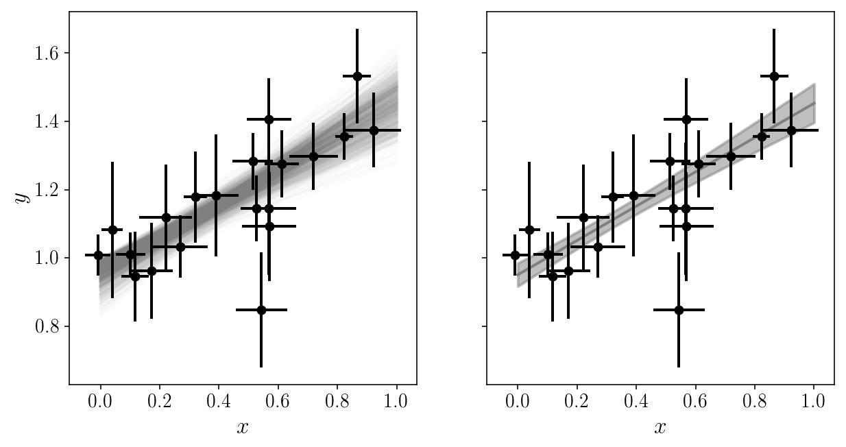
We got around the number of parameters by analytically marginalizing the ones we don’t really care about. Sometimes this is not possible!
Extensions (break out sessions?)
- Automatic differentiation with autograd, tensorflow, etc.
- Nested Sampling for nasty distributions and model comparison. Application: fitting multiple components/lines to a data set.
- Model testing, model comparison. I have multiple models. Which is the best? Example: fit multiple lines to data.
- Gibbs sampling: The default solution for population models.
- Large hierarchical models and high-dimensional parameters inference: Graphical representation of hierarchical models and parameter inference.
- Hamiltonian Monte Carlo with quasi-auto-tuning for millions of parameters. Application: fitting a line with many latent parameters (x noise, outliers, etc).
- Multi-stage hybrid sampling: Application: non-linear models with many parameters and complicated gradients.
- Connections to deep machine learning: Bayesian interpretation of Convolution networks, Adversarial training, deep forward models, etc. TensorFlow.
Let me know if you are interested and we will organize a session. A few notebooks and mode advanced examples available on https://ixkael.github.io
Final thoughts
With the right method you can solve problems/models that seem intractable. Don’t underestimate yourself! Start small, but be ambitious.

https://chi-feng.github.io/mcmc-demo/app.html