This is an extract from a notebook available at this location on Github.

We will make a simple hierarchical probabilistic model and illustrate:

• the shrinkage of uncertainties on individual objects in the presence of population parameters,
• the way the likelihood function must be modified to account for selection effects (here a cut on the signal-to-noise ratio of the data points),
• use Hamiltonian Monte Carlo to perform a very efficient parameter inference

Requirements

Some basic knowledge of Bayes theorem, parameter inference via MCMC, hierarchical probabilistic models, and Hamiltonian Monte Carlo.

Setup

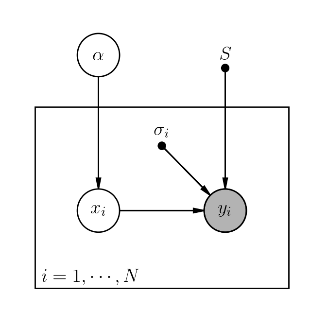
Our model will consist of:

• one population parameter \(\alpha\), describing the distribution of values \(x\) via \(p(x\vert \alpha)\),
• a set of \(N\) true (unobserverd, or latent) variables \(\{x_i\}_{i=1, \cdots, N}\) drawn from \(p(x\vert \alpha)\),
• a set of \(N\) noisy, observed variables \(\{y_i\}_{i=1, \cdots, N}\) drawn from \(p(y\vert x, sigma)\),
• a set of noise levels, described by \(\sigma_i\), which are given / fixed,
• a selection effect S, for example a cut on signal-to-noise ratio (SNR) applied to the noisy variables \(\{y_i\}\).

Let us draw the model corresponding to this description:

Parameter inference (without selection effects)

We want to infer \(\alpha\) and \(\{ x_i \}_{i=1, \cdots, N}\) from \(\{ y_i \}_{i=1, \cdots, N}\).

The posterior distribution on those parameters, via Bayes’ theorem applied to the hierarchical model, is:

\[p(\alpha, \{ x_i \} \vert \{ y_i \}, S) \propto p(\alpha) \prod_{i=1}^N p(x_i\vert \alpha)p(y_i\vert x_i)\]

The denominator (the evidence, or marginalized likelihood) can be dropped since it is constant w.r.t. the parameters of interest. We are only interested in exploring the interesting region of the posterior distribution, not its overall scale (which we would need for model comparison/selection).

\(p(y_i\vert x_i)\) is the likelihood function. \(p(x_i\vert \alpha)p\) is the population model, \(p(\alpha)\) the prior.

Parameter inference (with selection effects)

We now assume that the data \(\{ y_i \}_{i=1, \cdots, N}\) have been selected according to a selection effect or cut which will affect the parameters of interest (otherwise it would not affect any of the probabilisties and it could be dropped).

The posterior distribution on the parameters is now:

\[p(\alpha, \{ x_i \} \vert \{ y_i \}, S) \propto p(\alpha) \prod_{i=1}^N p(x_i\vert \alpha)p(y_i\vert x_i,S)\]

The term \(p(y_i\vert x_i,S)\) is a new likelihood function (a slight abuse of terminology), modified by selection effects:

\[p(y_i\vert x_i,S) = \frac{ p(S \vert y_i) p(y_i\vert x_i) }{ p(S \vert x_i ) }\]

The term \(p(S \vert y_i) = \frac{ p(y_i \vert S) p(S) }{p(y_i)}\) is constant. The real selection function is implemented in \(p(y_i \vert S)\).

The other term,

\(p(S \vert x_i ) = \int \mathrm{d}y^\prime_i p(S \vert y^\prime_i) p(y^\prime_i\vert x_i)\),

captures the way the original likelihood function is modified due to selection effects.

Example: Gaussian noise and SNR cut

In many cases, we will have

\(p(y_i\vert x_i,S) \propto \frac{ p(y_i\vert x_i) } { \int \mathrm{d}y^\prime_i p(y^\prime_i \vert S) p(y^\prime_i\vert x_i)}\),

when the selection effects are simple and deterministic.

We now consider a simple signal-to-noise ratio (SNR) cut, with some threshold \(C\):

\(p(y_i \vert S) = 1\) if \(y_i/\sigma_i > C\), otherwise \(0\).

We also consider Gaussian noise, so that the likelihood function is simply

\(p(y_i\vert x_i) = \mathcal{N}(y_i-x_i;\sigma_i)\).

With this deterministic cut, the correction term of interest, \(p( S \vert x_i )\), is a convolution:

\(p(S \vert x_i ) = \int_{C\sigma_i}^{\infty} \mathrm{d}y^\prime_i \mathcal{N}(y^\prime_i-x_i;\sigma_i)\),

leading to

\[p( S \vert x_i ) \propto 1 - \mathrm{erf}( \frac{C\sigma_i - x_i}{\sqrt{2}\sigma_i} )\]

So the final result, our new likelihood function for the hierarchical model, is

\[p(y_i\vert x_i,S) \propto \frac{ \exp(-\frac{1}{2}(\frac{y_i-x_i}{\sigma_i})^2) }{ 1 - \mathrm{erf}( \frac{C\sigma_i - x_i}{\sqrt{2}\sigma_i} ) }\]

where are have dropped irrelevant multiplicative constant terms everywhere.

Lets test that with a simulation!

Let’s generate \(x_i\)’s from a Gaussian centered at \(\alpha\), then add noise.

Let’s also apply a SNR cut, i.e. only keep objects that satisfy some SNR criterion.

We will infer \(\alpha\) (and the \(\{x_i\}_{i=1, \cdots, N}\)) with the framework presented above.

We will check that neglecting the selection effects leads to a biased answer, and that the formulae above correctly mitigates this bias.

nobj = 1000
alpha, sigma_alpha = 10, 1 # some arbitrary values
x_i = alpha + sigma_alpha * np.random.randn(nobj) # Gaussian draws
sigma_i = np.random.uniform(sigma_alpha, sigma_alpha * 2, size=nobj) # uniform draws
y_i = x_i + sigma_i * np.random.randn(nobj)  # Gaussian draws from N(x_i, sigma_i)
# some grid for computing and plotting p(x\vert alpha), here a Gaussian.
x_grid = np.linspace(np.min(y_i), np.max(y_i), 100)
p_x_alpha_grid = np.exp(-0.5*((x_grid-alpha)/sigma_alpha)**2)/\
    np.sqrt(2*np.pi)/sigma_alpha

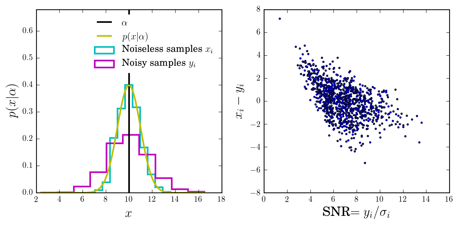
Let’s plot the initial distribution and the samples (with and without noise):

snrcut = 5 # our SNR cut
sel = np.where(y_i / sigma_i > snrcut)[0]
print(sel.size, "objects on", nobj, 'satisfy the SNR cut')

848 objects on 1000 satisfy the SNR cut

Let’s apply the SNR cut and visualise the resulting distribution of samples:

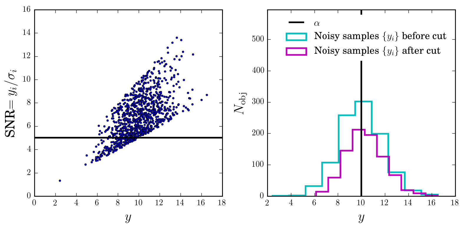
Intuition

We can already see that by applying the cut we are biasing ourselves towards higher values of \(\alpha\).

However, there is enough data (think coverage in \(x\) or \(y\)) and we the selection cut, so we could hope to invert this effect.

And indeed, the equations we derived above show that it is possible in theory.

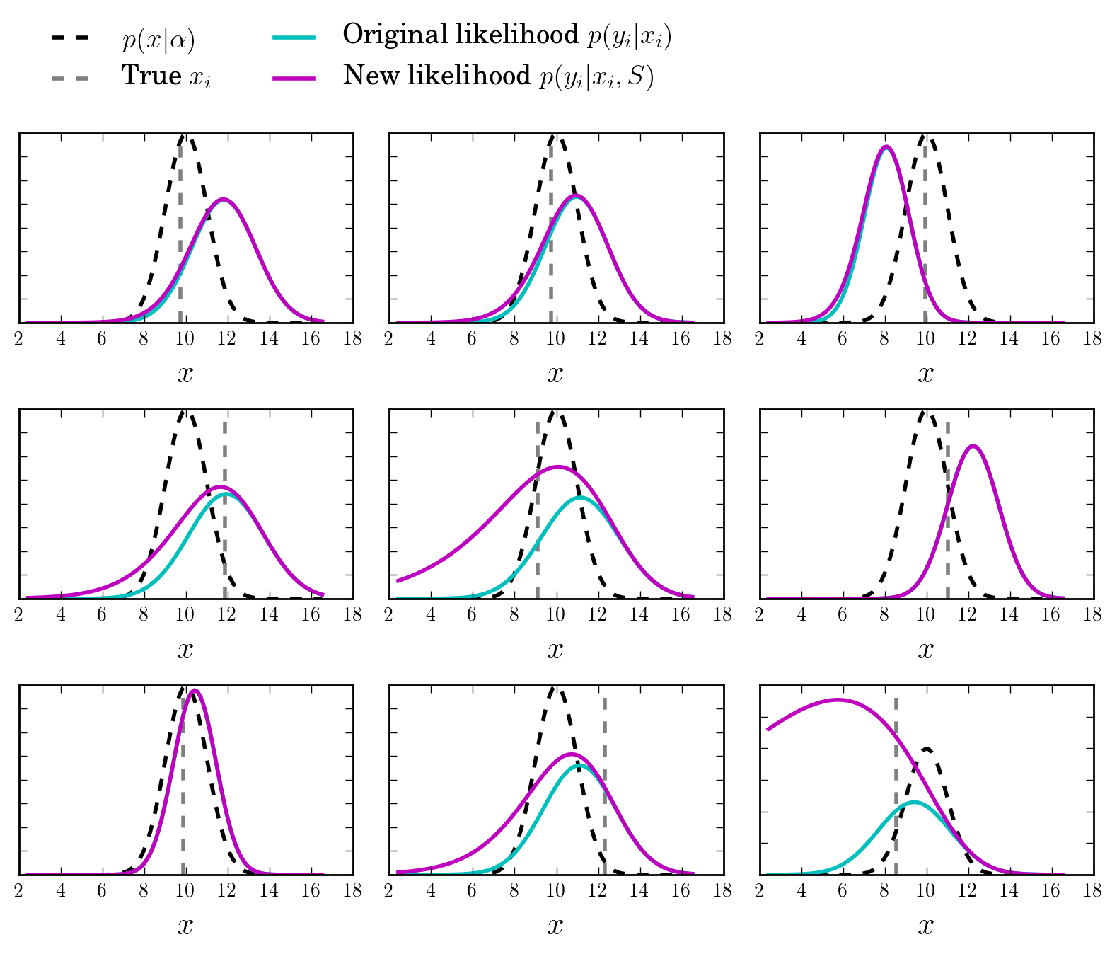
The new likelihoods

Let us now look at the new likelihood functions \(p(y_i\vert x_i, S)\) and compare them to the original ones, \(p(y_i\vert x_i)\), which ignore selection effects.

As expected, the correction term boosts the distribution at the low values of \(x\).

Sampling the posterior distributions via Hamiltonian Monte Carlo

Hamiltonian Monte Carlo (HMC) is a great technique for sampling from probability distributions of interest. It only requires the gradients w.r.t. the parameters of interest to be known analytically or easily computable.

Provided the HMC sampler is tuned, it is very efficient: it has an acceptance probability of one (it is an MCMC that never rejects samples) and efficiently mixes parameters, even in high dimensions.

Given that our model is very simple, has a lot of parameters, and admits simple gradients, it is very natural to opt for HMC to explore the posterior distributions of interest.

First run

Let’s run HMC to sample from the posterior distribution of the first model:

no SNR cut (use the full data set) with the correct likelihood function (with no SNR cut).

And check that the results make sense

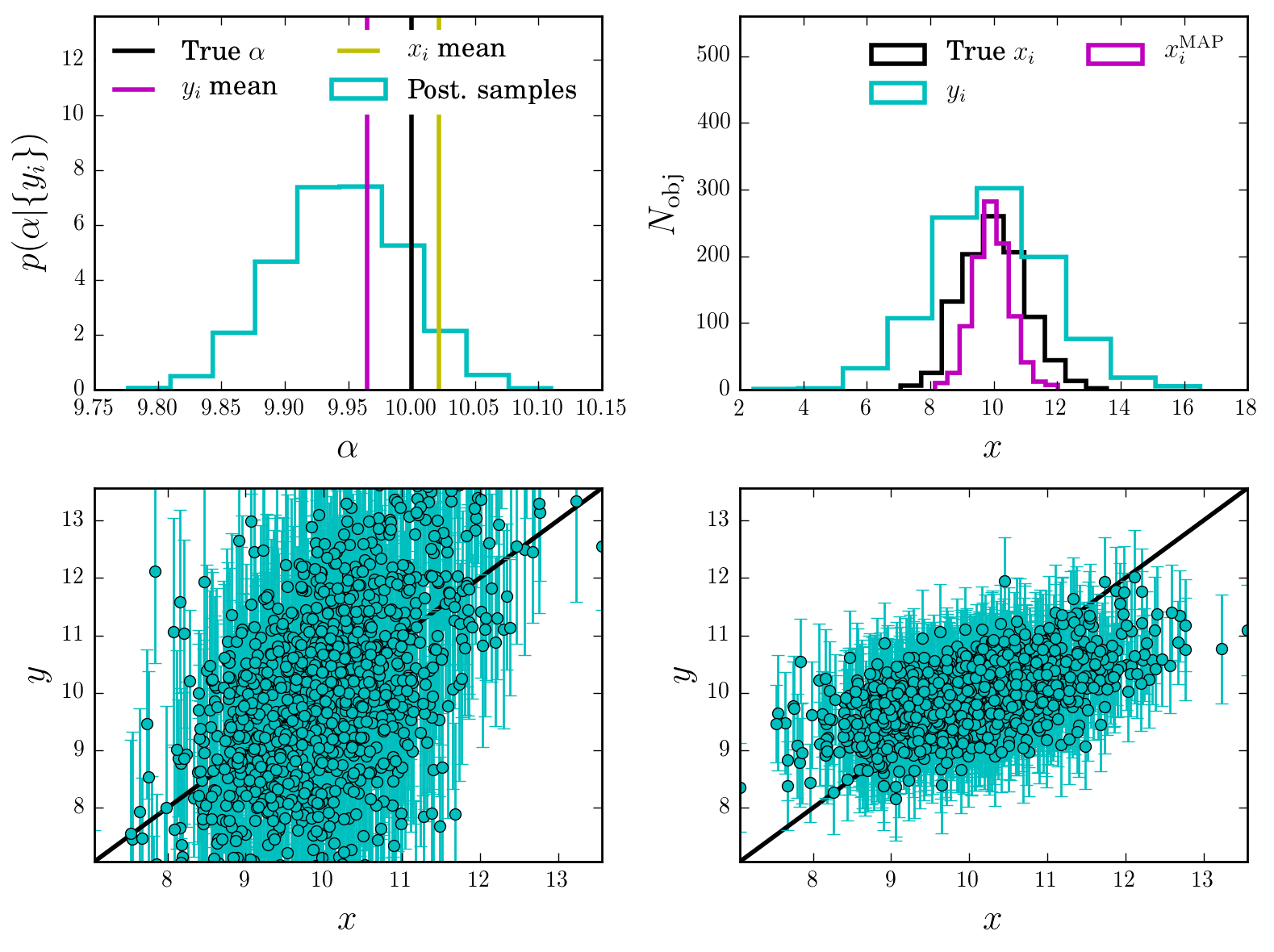
Interpretation

We see from the first panel that indeed the recover a nice posterior distribution for \(\alpha\) (with the \(\{ x_i \}\)s all marginalized out) capturing the true value.

The other panels show that the \(\{ x_i \}\) are also recover, and how the uncertainties significantly shrinkage around the true value, compared to the original likelihood \(p(y_i\vert x_i)\). All we have done is connecting them via the population model \(p(x\vert \alpha)\) and simultaneously infer all the parameters. This is a nice example of the typical Bayesian Shrinkage (tm) of uncertainties in hierarchical models.

Second and third runs

Let us now run the sampler on the subset of objects passing the SNR cut.

We will first do a run with the standard likelihood function ignoring selection effects.

We will then do an other run with the correct, selection-corrected likelihood function.

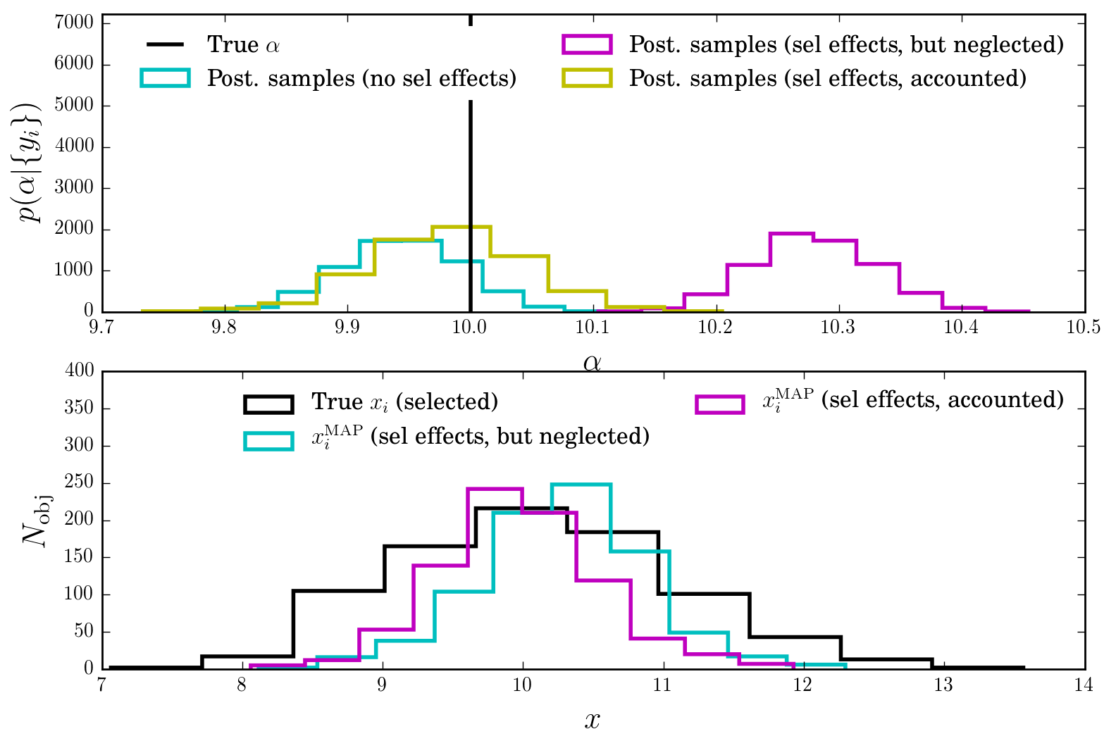
Interpretation

We see that indeed, running the standard likelihood on the SNR-selected objects leads to biased answers for \(\alpha\)!

This gets fixed when using the correct likelihood function, which is aware of the SNR cut and attempts to correct it.

Of course, this process has its limits. Here we have used enough data and our knowledge of the selection effect.

Conclusion

If you’ve applied cuts to your data, then you most likely have to modify the likelihood function involved in the parameter inference! This might require some math, but it will mitigate the bias arising from using an incorrect likelihood function.